Mike has a Cube, like this.

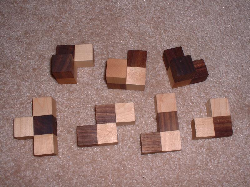
The cube is made of seven shapes, like these.
How many ways are there of assembling the cube? One could try placing each shape in turn in each position that it can occupy within the cube, and then seeing which of those combinations fill the cube. How many combinations of placements of pieces are there, then? For a very loose upper bound on this figure, assume that each of the seven shapes can be oriented against any of six faces of the cube, and in any of four directions relative to that, and can be translated to originate in any of the 27 cells in the cube. That gives (6 × 4 × 27)7 possibilities, which is 47,976,111,050,506,371,072.
But that's only a very loose bound. Many of the shapes have symmetries that mean that, after trying them one way round, there's no point in trying them the other way round - it'll just give the same answers. And none of the shapes can really be translated into all 27 different starting points without poking out of the sides of the cube, so that number can be replaced with a more accurate estimate too. Taking the symmetries and sizes of the seven shapes into account reduces the estimate to only about 40 million million possibilities.
There are about a million seconds in two weeks, so if a program can be written to check 40 million possibilities a second, then it'll only take two weeks to finish. On a 1GHz processor, checking 40 million possibilities a second requires a check to take on average 25 clock cycles. That seems doable enough to be worth investigating.
However, most of the work of checking possibilities can easily be avoided by noticing that, if any two pieces are placed in such a way that they would occupy the same space, then that definitely won't lead to any valid solutions. In other words, most of the possibilities will quickly turn out to be impossibilities. A program that can take advantage of that will probably finish in much less than two weeks.
One way to enumerate all the candidate shape placements is to enumerate all the placements of the first shape, then for each of those enumerate all the placements of the second shape, and then for each of those the placements of the third shape, and so on. In fact this approach allows exactly the work-avoiding strategy that is needed: when considering placing the Nth shape in a given position, look at whether that placement would conflict with the current positions of any of the N-1 shapes which have already been placed; if so, there is no need to continue investigating the positions of the remaining shapes. A solution is detected when all seven shapes have been placed, since that means each of the 27 cells in the shapes must be in different cells of the cube.
It's still worth thinking about how to check possible shape placements efficiently, though. One way to do it is to consider that a shape in a given position will fill some of the 27 cells of the cube and not others. So a partially-completed cube can be represented by a string of 27 bits, with a set bit indicating that the corresponding cell has been filled and a clear bit indicating that it is still free. And a choice of position for a particular shape can also be represented by a string of 27 bits, this time with the set bits indicating which of the cells will be filled by placing the shape in that position. Then, to see whether a new shape will fit into a partial solution in a given position, just check that the bit pattern for the partial solution and the bit pattern for the new shape placement have no set bits in common. And, to make a new partial solution with the new shape in its chosen place, just take the disjunction of those two bit patterns. Also, there aren't that many useful positions for each shape (between 64 and 144 in every case) so the bit patterns for each shape can be computed once to begin with and then reused.
Time to work this out in a Haskell module ...
There will definitely be a need for some bit-twiddling and other things.
There are seven shapes. The names here are intended to suggest their forms where possible. The P and Q shapes don't really look like any letter. They are mirror images of each other, though.
Each shape has a plan, which describes the cells of the cube that it occupies if placed in the left back corner of the bottom layer of the cube. The plan describes each row of each layer of the cube in turn, up to the point where all the remaining rows are empty. So the L plan can stop after only two rows, but the Y plan needs to go as far as the first row of the second layer.
The terminology 'form' is introduced to mean an assignment of shapes to positions in the cube. A form could be represented in all sorts of ways - 27 bits, or a string of 27 characters, or an array of booleans, or something else. A three-dimensional list of characters is slightly ugly, in that it is quite possible to construct forms that have the wrong dimensions or meaningless contents. But it has the advantage of allowing lots of built-in list manipulation and display functions to be brought to bear.
It's useful to be able to compare and sort forms. Again, the choice of representation allows different encodings of the same form to seem unequal when they shouldn't, but that isn't a problem in practice.
An easily readable representation of a form is helpful for listing the solutions (as well as for playing with individual shapes' forms to show that things are working properly). Transposing the layers of rows allows the successive layers to be printed next to one another instead of above one another to make better use of screen space - an example of the list representation making things easier.
There is an empty form (corresponding to the partial solution where no shapes have been placed yet) and it's easy to see how to combine a form with another form and that (if the combination is valid) this will be a symmetric operation, so these forms naturally produce a Monoid.
To compute the bit pattern for a form, string the characters for each of its rows together and then convert each character in turn into a single bit.
It'll be useful to know how many cells of the cube are occupied by a given form.
As mentioned before, the plan of each shape describes the cells it occupies when pushed into a particular corner of the cube. Here is a way to take this plan (which doesn't even describe the entire cube!) and turn it into a complete form suitable for combining with other forms.
Translation functions take a form for a shape, and give a form for the same shape but shifted by one place along one of the three axes. Because the default forms of the shapes are always in one particular corner, these translation functions only need to cover shifts away from that one corner in order to be able to describe all the possible positions into which the shape can be translated.
These functions implicitly fix the coordinate system of the form representation: a list of layers, each of which is a list of rows, each of which is a list of cells. This means, for example, that manipulating the outermost list of the structure corresponds to dealing with the cube layer-wise.
Each of these functions inserts empty space on one face of the cube and chops one slice of cells off the opposite face of the cube. Again, the list representation makes them easy to define.
The rotation functions are slightly more complicated. For convenience, they are based on a 90-degree rotation being equivalent to a transposition followed by a reflection.
Rotation about the X axis leaves each row unchanged, so it's just the rotation applied to the outer two layers of lists.
To rotate about the Y axis, first transpose Z and Y to bring the Z and X axes next to each other, then apply the rotation to those Z and X axes, then transpose Y and Z to restore the coordinate system. Note that the direction of the applied rotation is reversed because transposition reverses the chirality of the representation.
Finally, to rotate about Z, apply the desired rotation to each layer in turn.
These translation and rotation functions are a basis for enumerating all the forms that a shape can produce. As discussed earlier, each shape can be rotated to have its base against one of six faces of the cube ...
... and then rotated in the plane of that face in one of four ways ...
... and then translated by up to two cells in each of three directions, but only so long as the shape still lies within the bounds of the cube.
So, all the forms that a shape can have can be listed by applying each combination of major rotation, minor rotation and shift to the default form for the shape. Some of these will be duplicates because of the symmetries of the shape. nub is used to eliminate them, which is quite inefficient but this only needs to be computed once for each shape.
As described so far, combining these lists of forms will give 48 times more solutions than are interesting, because every solution that is merely the rotation or reflection of another solution will also be found. An easy way to avoid that is to fix the orientation of one of the shapes - say, the first one. Then, there can't be any solutions that are simply rotations of another solution, because that one piece is always facing the same way. Similarly, omit any translations for it that give any forms which are mirror images. These considerations reduce the forms for the L shape to just four.
For each shape, all the forms it can have and their bit representations. Keeping this list on its own avoids computing a shape's forms and their bit representations afresh for each new partial solution in which the shape is being considered.
For each shape in turn, add each of its forms in turn into the partial solutions found so far, but only if the bit patterns for the form and the partial solution don't overlap.
Finally, print out all the solutions, separated by newlines.
An optimised build of this program is easily fast enough:
(These times are from a system with dual 2.5GHz hyperthreaded Intel Core i5 CPUs.)
Naturally, the Soma cube (for that is what it is) has been studied thoroughly already.
It will be interesting to see what optimisations the compiler has found and what the structure of the optimised program looks like. It will also be interesting to see what a comparable program in C or C++ or Python would look like, and how fast they go.
The cube is made of seven shapes, like these.
How many ways are there of assembling the cube? One could try placing each shape in turn in each position that it can occupy within the cube, and then seeing which of those combinations fill the cube. How many combinations of placements of pieces are there, then? For a very loose upper bound on this figure, assume that each of the seven shapes can be oriented against any of six faces of the cube, and in any of four directions relative to that, and can be translated to originate in any of the 27 cells in the cube. That gives (6 × 4 × 27)7 possibilities, which is 47,976,111,050,506,371,072.
But that's only a very loose bound. Many of the shapes have symmetries that mean that, after trying them one way round, there's no point in trying them the other way round - it'll just give the same answers. And none of the shapes can really be translated into all 27 different starting points without poking out of the sides of the cube, so that number can be replaced with a more accurate estimate too. Taking the symmetries and sizes of the seven shapes into account reduces the estimate to only about 40 million million possibilities.
There are about a million seconds in two weeks, so if a program can be written to check 40 million possibilities a second, then it'll only take two weeks to finish. On a 1GHz processor, checking 40 million possibilities a second requires a check to take on average 25 clock cycles. That seems doable enough to be worth investigating.
However, most of the work of checking possibilities can easily be avoided by noticing that, if any two pieces are placed in such a way that they would occupy the same space, then that definitely won't lead to any valid solutions. In other words, most of the possibilities will quickly turn out to be impossibilities. A program that can take advantage of that will probably finish in much less than two weeks.
One way to enumerate all the candidate shape placements is to enumerate all the placements of the first shape, then for each of those enumerate all the placements of the second shape, and then for each of those the placements of the third shape, and so on. In fact this approach allows exactly the work-avoiding strategy that is needed: when considering placing the Nth shape in a given position, look at whether that placement would conflict with the current positions of any of the N-1 shapes which have already been placed; if so, there is no need to continue investigating the positions of the remaining shapes. A solution is detected when all seven shapes have been placed, since that means each of the 27 cells in the shapes must be in different cells of the cube.
It's still worth thinking about how to check possible shape placements efficiently, though. One way to do it is to consider that a shape in a given position will fill some of the 27 cells of the cube and not others. So a partially-completed cube can be represented by a string of 27 bits, with a set bit indicating that the corresponding cell has been filled and a clear bit indicating that it is still free. And a choice of position for a particular shape can also be represented by a string of 27 bits, this time with the set bits indicating which of the cells will be filled by placing the shape in that position. Then, to see whether a new shape will fit into a partial solution in a given position, just check that the bit pattern for the partial solution and the bit pattern for the new shape placement have no set bits in common. And, to make a new partial solution with the new shape in its chosen place, just take the disjunction of those two bit patterns. Also, there aren't that many useful positions for each shape (between 64 and 144 in every case) so the bit patterns for each shape can be computed once to begin with and then reused.
Time to work this out in a Haskell module ...
> module Cube whereThere will definitely be a need for some bit-twiddling and other things.
> import Data.Bits
> import Data.List (intercalate, nub, transpose, unfoldr)
> import Data.Monoid
> import Data.Word
There are seven shapes. The names here are intended to suggest their forms where possible. The P and Q shapes don't really look like any letter. They are mirror images of each other, though.
> data Shape = L | S | T | R | P | Q | Y
>   deriving (Enum, Show)
Each shape has a plan, which describes the cells of the cube that it occupies if placed in the left back corner of the bottom layer of the cube. The plan describes each row of each layer of the cube in turn, up to the point where all the remaining rows are empty. So the L plan can stop after only two rows, but the Y plan needs to go as far as the first row of the second layer.
> plan L = "XXX" ++
>          "X  "
> plan S = " XX" ++
> "XX "> plan T = "XXX" ++
> " X "> plan R = "XX " ++
> "X "> plan P = "X " ++
> "X " ++
> " " ++
> "XX "> plan Q = " X " ++
> " X " ++
> " " ++
> "XX "> plan Y = "XX " ++
> "X " ++
> " " ++
> "X "The terminology 'form' is introduced to mean an assignment of shapes to positions in the cube. A form could be represented in all sorts of ways - 27 bits, or a string of 27 characters, or an array of booleans, or something else. A three-dimensional list of characters is slightly ugly, in that it is quite possible to construct forms that have the wrong dimensions or meaningless contents. But it has the advantage of allowing lots of built-in list manipulation and display functions to be brought to bear.
> newtype Form = Form [[[Char]]]
> unform (Form x) = x
It's useful to be able to compare and sort forms. Again, the choice of representation allows different encodings of the same form to seem unequal when they shouldn't, but that isn't a problem in practice.
> instance Eq Form where
>   (Form x) == (Form y) = x == y
> instance Ord Form where
> Form x `compare` Form y = x `compare` yAn easily readable representation of a form is helpful for listing the solutions (as well as for playing with individual shapes' forms to show that things are working properly). Transposing the layers of rows allows the successive layers to be printed next to one another instead of above one another to make better use of screen space - an example of the list representation making things easier.
> instance Show Form where
>   show (Form f) = unlines [showSlice s | s <- transpose f]
>    where
>     showSlice s = intercalate "  " [ showRow r | r <- s ]
>     showRow r = "|" ++ r ++ "|"
There is an empty form (corresponding to the partial solution where no shapes have been placed yet) and it's easy to see how to combine a form with another form and that (if the combination is valid) this will be a symmetric operation, so these forms naturally produce a Monoid.
> instance Monoid Form where
>   mempty = Form $ (replicate 3 . replicate 3 . replicate 3) ' '
>   mappend (Form x) (Form y) = Form $ (zipWith . zipWith . zipWith)
>                                      superpose x y
>    where
>     superpose ' ' ' ' = ' '
>     superpose  a  ' ' =  a
>     superpose ' '  b  =  b
>     superpose  _   _  = '#'  -- This should never happen!
To compute the bit pattern for a form, string the characters for each of its rows together and then convert each character in turn into a single bit.
> flatten = concat . concat . unform
> asBits :: Form -> Word32
> asBits f = sum [bit n | (n, x) <- zip [0..] (flatten f), x /= ' ']
It'll be useful to know how many cells of the cube are occupied by a given form.
> size f = length [x | x <- flatten f, x /= ' ']As mentioned before, the plan of each shape describes the cells it occupies when pushed into a particular corner of the cube. Here is a way to take this plan (which doesn't even describe the entire cube!) and turn it into a complete form suitable for combining with other forms.
> defaultForm :: Shape -> Form
> defaultForm shape = Form layers
>  where
>   layers = (inThrees . inThrees) fullPlan
>   fullPlan = [formChar c | c <- plan shape] ++
>              replicate (27 - length (plan shape)) ' '
>   inThrees = takeWhile (not . null) . unfoldr (Just . splitAt 3)
>   formChar ' ' = ' '
>   formChar  _  = head (show shape)
Translation functions take a form for a shape, and give a form for the same shape but shifted by one place along one of the three axes. Because the default forms of the shapes are always in one particular corner, these translation functions only need to cover shifts away from that one corner in order to be able to describe all the possible positions into which the shape can be translated.
These functions implicitly fix the coordinate system of the form representation: a list of layers, each of which is a list of rows, each of which is a list of cells. This means, for example, that manipulating the outermost list of the structure corresponds to dealing with the cube layer-wise.
Each of these functions inserts empty space on one face of the cube and chops one slice of cells off the opposite face of the cube. Again, the list representation makes them easy to define.
> tx (Form f) = Form [[[' ', a, b] | [a, b, _] <- layer] | layer <- f]
> ty (Form f) = Form [["   ", a, b] | [a, b, _] <- f]
> tz (Form [a, b, _]) = Form [replicate 3 "   ", a, b]
The rotation functions are slightly more complicated. For convenience, they are based on a 90-degree rotation being equivalent to a transposition followed by a reflection.
> cw = transpose . reverse
> ccw = reverse . transpose
Rotation about the X axis leaves each row unchanged, so it's just the rotation applied to the outer two layers of lists.
> withForm f = Form . f . unform
> rx = withForm ccw
> rx' = withForm cw
To rotate about the Y axis, first transpose Z and Y to bring the Z and X axes next to each other, then apply the rotation to those Z and X axes, then transpose Y and Z to restore the coordinate system. Note that the direction of the applied rotation is reversed because transposition reverses the chirality of the representation.
> ry = withForm (transpose . map ccw . transpose)
> ry' = withForm (transpose . map cw . transpose)
Finally, to rotate about Z, apply the desired rotation to each layer in turn.
> rz = withForm (map cw)
> rz' = withForm (map ccw)
These translation and rotation functions are a basis for enumerating all the forms that a shape can produce. As discussed earlier, each shape can be rotated to have its base against one of six faces of the cube ...
> majors = [id, ry, (ry . ry), ry', rz, rz']... and then rotated in the plane of that face in one of four ways ...
> minors = [id, rx, (rx . rx), rx']... and then translated by up to two cells in each of three directions, but only so long as the shape still lies within the bounds of the cube.
> shifts shape = [t | t <- [times x tx . times y ty . times z tz |
>                           x <- [0..2],
>                           y <- [0..2],
>                           z <- [0..2]], inBounds t]
>  where
>   inBounds t = size (t (defaultForm shape)) == size (defaultForm shape)
>   times 0 f = id
>   times n f = f . times (n-1) f
So, all the forms that a shape can have can be listed by applying each combination of major rotation, minor rotation and shift to the default form for the shape. Some of these will be duplicates because of the symmetries of the shape. nub is used to eliminate them, which is quite inefficient but this only needs to be computed once for each shape.
As described so far, combining these lists of forms will give 48 times more solutions than are interesting, because every solution that is merely the rotation or reflection of another solution will also be found. An easy way to avoid that is to fix the orientation of one of the shapes - say, the first one. Then, there can't be any solutions that are simply rotations of another solution, because that one piece is always facing the same way. Similarly, omit any translations for it that give any forms which are mirror images. These considerations reduce the forms for the L shape to just four.
> allForms :: Shape -> [Form]
> allForms shape = nub $ [t (defaultForm shape) | t <- transforms shape]
>  where
>   transforms L = [id, ty, tz, (ty . tz)]
>   transforms shape =  [maj . min . shift |
>                        maj <- majors,
>                        min <- minors,
>                        shift <- shifts shape]
For each shape, all the forms it can have and their bit representations. Keeping this list on its own avoids computing a shape's forms and their bit representations afresh for each new partial solution in which the shape is being considered.
> combos = [[(f, asBits f) | f <- allForms shape] | shape <- enumFrom L]For each shape in turn, add each of its forms in turn into the partial solutions found so far, but only if the bit patterns for the form and the partial solution don't overlap.
> solutions = map fst $ foldr1 addForm combos where
>   addForm partialSolution form = [(pf `mappend` f, pb .|. b) |
>                                   (f, b) <- form,
>                                   (pf, pb) <- partialSolution,
>                                   pb .&. b == 0]
Finally, print out all the solutions, separated by newlines.
> main = putStrLn $ intercalate "\n" [show s | s <- solutions]An optimised build of this program is easily fast enough:
$ ghc --make -O2 -main-is Cube Cube.lhs
[1 of 1] Compiling Cube             ( Cube.lhs, Cube.o )
Linking Cube ...
$ time ./Cube > solutions.txt

real    0m1.239s
user    0m1.229s
sys 0m0.008s
(These times are from a system with dual 2.5GHz hyperthreaded Intel Core i5 CPUs.)
Naturally, the Soma cube (for that is what it is) has been studied thoroughly already.
It will be interesting to see what optimisations the compiler has found and what the structure of the optimised program looks like. It will also be interesting to see what a comparable program in C or C++ or Python would look like, and how fast they go.
No comments:
Post a Comment